BLDC: From Basic Physics to Control Theory
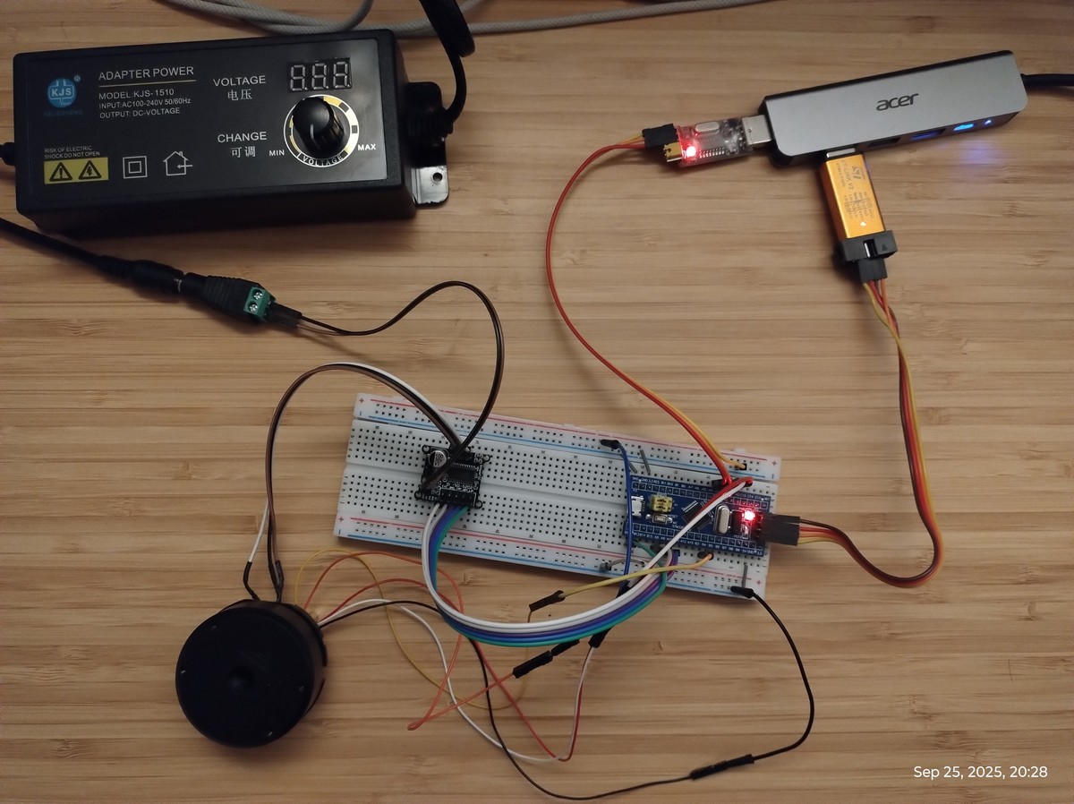 My BLDC Experiment Setup
I learned that the joints in robots are mainly using BLDC motor + FOC control. To have a better understanding, I bought two sets of small BLDC + MT6701 magnetic encoder + SimpleFOC mini board during this summear holiday in China. One set cost about 10 euros and it brings so much fun to try and learn. I have already put my code and experiments in this repo. In this article I document the theory part of what I have learnd with the help of ChatGPT.
1. What Is a BLDC Motor?
Brushless DC motors (BLDC motors) have quietly become one of the most important actuators of the modern world. They power drones, electric vehicles, camera gimbals, cooling fans, and increasingly, robotics of every scale. Despite the name, BLDC motors are not direct descendants of brushed DC motors—they are closer to small synchronous AC machines with permanent magnets, but driven by electronics that emulate DC motor behavior.
Traditionally, a DC motor uses brushes and a commutator: a mechanical switch that changes the current direction inside the rotor as it spins. This guarantees that torque always pushes in the correct direction. A BLDC motor removes the brushes and the commutator entirely. Instead of switching current mechanically, the motor relies on an electronic controller that energizes the stator windings in the correct sequence.
The rotor contains permanent magnets; the stator has a set of coils. By energizing these coils in the right order, we create a rotating magnetic field that “pulls” the rotor around. Because there are no brushes touching a commutator, BLDC motors have higher lifetime, efficiency, and speed.
Electrically, BLDC motors can be driven in different ways:
Trapezoidal BLDC: The controller energizes each phase in a 6-step sequence. The currents are ideally trapezoidal. This is simple to implement and very common in cost-sensitive high-volume products.
Sinusoidal BLDC (PMSM): The currents are sinusoidal and matched to the rotor position. This produces smoother torque, better efficiency, and quieter operation. This style of motor is technically a permanent-magnet synchronous motor (PMSM). It is often used in EVs, drones, and high-end robotics.
Even though the hardware is often the same, the drive method makes the difference. In this article, whenever we say “BLDC,” we mean the sinusoidal, FOC-driven type—a PMSM.
1.1. Inrunner and Outrunner
A BLDC motor comes in two common mechanical forms: inrunners and outrunners.
Inrunner The rotor (magnets) is inside, the stator (coils) is outside. Typical in high-speed motors and industrial actuators.
Outrunner The rotor is the outer shell containing magnets, and it spins around a stationary stator at the center. This design produces higher torque because the magnets are farther from the rotation axis, increasing the lever arm.
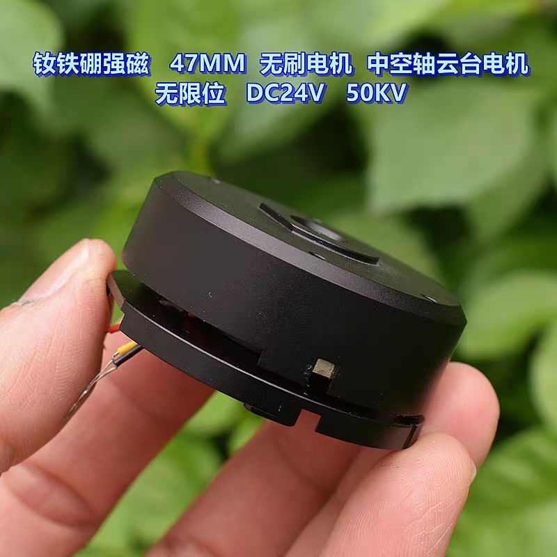
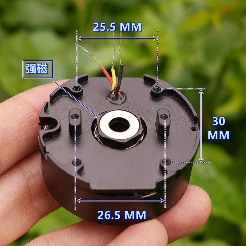
In robots outrunners are typically used. Therefore we’ll use that as our mental model. An outrunner contains:
- A stator with multiple teeth (slots) wrapped in copper wire
- A rotating bell housing containing permanent magnets
- Back-iron (part of both stator and rotor), which guides magnetic flux
- Bearings, which support the spinning bell
- A central shaft
Despite looking simple from the outside, the magnetic and mechanical optimization inside an outrunner is highly sophisticated.
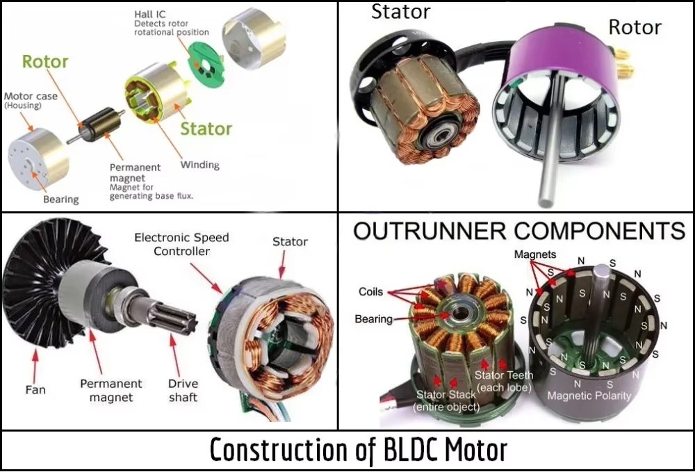 BLCD construction
1.2. Poles, Slots, and Coils
Poles and Pole-Pairs
A rotor’s magnets are arranged in alternating north–south pairs around the circumference. Each N–S pair forms one pole-pair, and pole-pairs define the relationship between electrical and mechanical speeds:
- 1 mechanical revolution = $p$ electrical revolutions
- Electrical frequency = $p$ × mechanical frequency
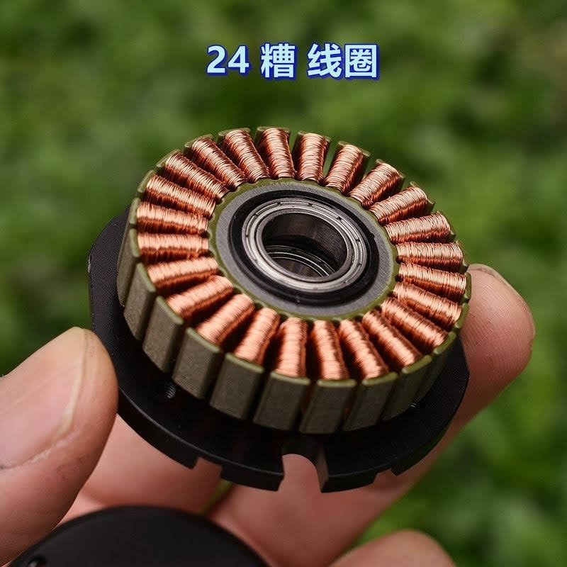
Stator Slots
The stator has multiple “teeth,” called slots. Each slot can contain one or more sets of coils. The number of slots and the number of poles determine the winding pattern.
Example: A popular configuration is 12 slots, 14 poles (12s14p).
Concentrated vs. Distributed Winding
Concentrated winding Each coil is concentrated around one stator tooth. Common in outrunners.
Distributed winding The same phase’s coils are spread over multiple slots. Common in industrial motors.
Balanced vs. Unbalanced Winding Patterns
A balanced winding ensures that in every repeating segment of the motor:
- Each phase has the same total number of coils
- Torque ripple is minimized
- The motor runs efficiently and vibration-free
Designs like 12-slot 14-pole or 9-slot 12-pole are well-known balanced configurations.
Design Pointers & References
The choice of slot/pole combination has huge impact on:
- Torque ripple
- Cogging torque
- Efficiency
- Manufacturability
- Smoothness of rotation
Engineers use established combinations such as 12s14p, 9s12p, 18s16p, etc. The design space is surprisingly deep.
A very good introductory reference is:
“Selecting the best pole and slot combination for a BLDC (PMSM) motor with concentrated windings” https://things-in-motion.blogspot.com/2019/01/selecting-best-pole-and-slot.html
It explains why certain slot/pole pairs work well and others produce unwanted magnetic imbalances.
1.3. Magnetic Circuit Elements
Back-Iron
The stator and rotor cores are made of laminated steel. The back-iron (also called the yoke) helps close the magnetic flux loop through the motor. Stronger back-iron allows the magnetic field to flow efficiently, reducing losses and improving torque.
Halbach Array
Some high-end BLDC motors use a Halbach array in the rotor. This is a special magnet arrangement where the magnetization rotates around the circumference, concentrating magnetic flux on one side and reducing it on the other. Most hobby outrunners do not use full Halbach arrays due to cost, but partial Halbach patterns are becoming more common.
1.4. Three-Phase Windings
A BLDC/PMSM stator has three electrically distinct phases: A, B, and C, each driven 120° apart in electrical angle as:
\[\begin{aligned} i_a(t) &= I\sin(\omega t),\\ i_b(t) &= I\sin\!\left(\omega t - \tfrac{2\pi}{3}\right),\\ i_c(t) &= I\sin\!\left(\omega t + \tfrac{2\pi}{3}\right). \end{aligned}\]The coils are physically interleaved around the stator but electrically connected to form three balanced phases. ABC ABC ABC … repeated around the stator. Together they produce a rotating magnetic field.
2. Basic Electromagnetic Physics
Before diving into control theory, it helps to revisit some of the essential physics behind BLDC motors. These ideas—magnetic dipoles, flux, torque—are not only elegant but surprisingly intuitive once you visualize them inside the motor.
2.1. Magnetic Dipoles & Flux
Coil Current → Magnetic Dipole Moment
Whenever a current flows through a loop of wire, it creates a magnetic dipole. The strength and orientation of this magnetic “arrow” is described by the dipole moment:
\[\mathbf{\mu} = N I \mathbf{A}\]- $N$: number of turns
- $I$: current
- $\mathbf{A}$: area of the loop (Direction: given by the right-hand rule)
In a BLDC motor, the stator coils create magnetic dipoles that interact with the magnets on the rotor. By controlling the phase currents, we control these magnetic dipoles in time and space.
Permanent-Magnet Rotor Flux
The rotor contains permanent magnets, which create their own magnetic field. Instead of expressing this field as a simple dipole moment, motor engineers often use the term flux linkage, written: $\psi_f$.
Flux linkage describes how much magnetic flux from the rotor passes through each stator phase. It is a key parameter in BLDC/PMSM models.
Physically, it is the “magnetic fingerprint” of the rotor that the stator interacts with to produce torque.
2.2. Torque Generation
Torque in electric motors can be understood from two complementary viewpoints:
Lorentz-Force View
A current-carrying conductor in a magnetic field experiences a force:
\[\mathbf{F} = I \mathbf{L} \times \mathbf{B}\]- $I$: current
- $\mathbf{L}$: vector length of conductor
- $\mathbf{B}$: magnetic field
Arrange many such conductors around a rotor and you get torque that tends to spin the rotor.
Magnetic-Dipole View
A magnetic dipole in a magnetic field experiences a torque trying to align it:
\[\boldsymbol{\tau} = \boldsymbol{\mu} \times \mathbf{B}\]This view is simpler and more intuitive: the stator’s dipoles are trying to align the rotor’s magnetic field with them. If the stator field is always rotated slightly ahead of the rotor, the rotor continually chases it—producing rotation.
Why We Do Not Compute PMSM/BLDC Torque Using These Two Views
While the Lorentz-force and magnetic-dipole perspectives are physically correct, they are not practical for deriving torque in AC machines. A PMSM/BLDC motor has:
- distributed three-phase windings,
- a rotating magnetic field,
- flux linkages that depend on rotor position,
- possible saliency ($L_d \neq L_q$),
- and airgap fields that are spatially sinusoidal.
Directly computing torque from $\mathbf{F} = I \mathbf{L} \times \mathbf{B}$ or $\boldsymbol{\mu} \times \mathbf{B}$ would require integrating forces or dipole interactions around the entire airgap with accurate field distributions. This is mathematically complex and does not yield the clean expressions used in control.
Because of this, Field-Oriented Control (FOC) instead relies on power balance:
\[\tau_e = \frac{p_e}{\omega_m}.\]Electrical power $p_e$ is easy to compute, and substituting it into the above relation directly yields the standard PMSM BLDC torque equation:
\[\tau_e = \frac{3}{2} p(\psi_d i_q - \psi_q i_d).\]This approach avoids complicated field integrations and fits perfectly with how the motor is controlled in practice. We will get back to this later.
2.3. Electrical vs. Mechanical Quantities
A BLDC/PMSM effectively operates in two domains simultaneously:
Mechanical Speed
The angular speed of the rotation of the rotor: $\omega_m$ (rad/s or RPM).
(Optimal) Electrical Speed
The optimal angular speed of the AC currents driving the stator:
\[\omega_e = p \omega_m\]The factor $p$ (pole pairs) means the electrical world spins faster than the mechanical world. For a common 14-pole (7-pole-pair) outrunner:
- If the rotor spins at 1,000 RPM
- The electrical field must rotate at 7,000 RPM
This multiplication is essential to understand controller timing, FOC synchronization, and speed estimation.
Actually, I find the term “electrical speed” somewhat misleading. I would instead call it “magnetic speed” or “optimal electrical speed” since FOC attempts to match the electrical speed to that value.
2.4. Back-EMF and Sensorless Sensing
What Is Back-EMF?
As the rotor magnets sweep past the stator coils, they induce a voltage. This voltage is called back electromotive force, or back-EMF:
\[e = -N \frac{d\Phi}{dt}\]- If the rotor moves faster, the flux changes faster, and back-EMF increases.
- Back-EMF opposes the applied voltage, reducing net current at high speeds.
Back-EMF is why open-loop voltage control cannot maintain torque at high RPM—it simply loses headroom.
Zero-Crossing in Trapezoidal BLDC
In 6-step trapezoidal BLDC, controllers often use a simple sensorless method:
- Measure the undriven phase
- Detect when its back-EMF crosses zero
- Commutate 60° later
This works surprisingly well for hobby ESCs, fans, and pumps.
Why It Fails for Sinusoidal FOC
For smooth sinusoidal control, simple zero-crossing is insufficient:
- Currents are sinusoidal, not 6-step
- Back-EMF must be measured continuously
- The controller needs the electrical angle, not just 60° intervals
- Noise and PWM switching corrupt zero-crossing detection
FOC requires much more precise rotor position: often ±1° electrical accuracy. This is why FOC systems use:
- Encoders
- Hall sensors with interpolation
- High-frequency injection
- Flux observers (e.g., sliding-mode, Kalman-style)
Back-EMF still matters—but now it is part of a detailed observer model rather than a simple switching cue.
3. From Physics to Control Theory
Up to now we’ve looked at the physical structure of a BLDC motor and the magnetic interaction that produces torque. The next step is understanding how modern controllers turn these physical laws into smooth, precise, and efficient motion. This is where the elegance of mathematics enters: transforms, rotating frames, and feedback loops that together make a BLDC behave almost exactly like a brushed DC motor—but without the brushes.
3.1. Why We “Want a DC Motor” Behavior
A brushed DC motor is surprisingly easy to control. Its torque is directly proportional to current:
\[T = k_t I\]The commutator inside the motor ensures that this torque always pushes in the correct direction. The user simply applies a voltage and gets smooth torque. No angle tracking, no phase switching, no sinusoidal waveforms.
A BLDC (or PMSM), by contrast, has:
- Three phases (which has its own design reason)
- Rotating magnetic fields
- Strong coupling between flux, torque, and position
- Electrical and mechanical speeds that differ
This makes direct control difficult—unless we introduce mathematical tools that simplify everything.
The Big Idea
If we transform the motor’s three-phase AC currents into a different coordinate system where torque and flux appear as independent channels—just like a DC motor—then we can control a BLDC with simple controllers while enjoying the benefits of brushless technology.
This idea was first explored by Robert H. Park in 1929, who discovered that expressing AC machine currents in a rotor-synchronous reference frame eliminates the sinusoidal time-varying terms. Later, Edith Clarke in 1938 introduced what is now called the Clarke transform, completing the mapping from three-phase quantities to a two-phase stationary reference frame. These ideas form the foundation of vector control and eventually field-oriented control (FOC).
3.2. Clarke Transform (abc → αβ)
A BLDC’s stator has three phase currents: $i_a,\ i_b,\ i_c$. In a balanced system they are $120^\circ$ apart and satisfy \(i_a + i_b + i_c = 0.\)
Clarke’s transform maps these three currents to a two-dimensional vector in a stationary $\alpha\beta$ reference frame:
\[\begin{bmatrix} i_\alpha \\ i_\beta \end{bmatrix} = \frac{2}{3} \begin{bmatrix} 1 & -\tfrac{1}{2} & -\tfrac{1}{2} \\ 0 & \tfrac{\sqrt{3}}{2} & -\tfrac{\sqrt{3}}{2} \end{bmatrix} \begin{bmatrix} i_a \\ i_b \\ i_c \end{bmatrix}.\]This removes redundancy (since $i_a + i_b + i_c = 0 = i_\gamma$).
After Clarke’s transform we obtain
\[i_\alpha(t) = I \cos(\omega t), \qquad i_\beta(t) = I \sin(\omega t).\]This shows that the three sinusoidal phase currents collapse into a single vector of the same constant magnitude $I$ rotating at the same electrical frequency $\omega$. Instead of handling three phase waveforms, we track one circular trajectory in the $\alpha\beta$ plane.
Note here we use amplitude-invariant form of Clark transformation which gives:
\[i_a^2 + i_b^2 + i_c^2 = \frac{3}{2}\bigl(i_\alpha^2+i_\beta^2\bigr)\]and instantaneous electrical power satisfies
\[p_e = v_a i_a + v_b i_b + v_c i_c = \frac{3}{2}\bigl(v_\alpha i_\alpha + v_\beta i_\beta\bigr),\]where the voltages $v_\alpha$ and $v_\beta$ are tranformed using the same transformation matrix above.
3.3. Park Transform (αβ → dq)
The Park transform is the step that turns AC into DC—but only when viewed from the right coordinate system.
The rotor’s electrical angle is:
\[\theta_e = p \theta_m\]This is the angle of the rotor flux relative to the stator. If we rotate our coordinate axes by exactly this angle, then in this new rotating frame the currents stop oscillating.
Mathematically, the Park transform rotates the αβ vector into the dq frame:
\[\begin{bmatrix} i_d\\[4pt] i_q \end{bmatrix} = \begin{bmatrix} \cos\theta_e & \sin\theta_e\\[4pt] -\sin\theta_e & \cos\theta_e \end{bmatrix} \begin{bmatrix} i_\alpha\\[4pt] i_\beta \end{bmatrix}\]Physically,
- $i_d$ is the component of the stator current aligned with the rotor’s magnetic field (flux-producing).
- $i_q$ is the component perpendicular to the rotor’s magnetic field (torque-producing).
Substituting the $\alpha\beta$ expressions from Clark transformation into the Park transform and using the trigonometric identities
\[\begin{aligned} \cos(A - B) &= \cos A \cos B + \sin A \sin B, \\ \sin(A - B) &= \sin A \cos B - \cos A \sin B, \end{aligned}\]we get
\[\begin{aligned} i_d(t) &= I \cos\big(\omega t - \theta_e\big),\\[2pt] i_q(t) &= I \sin\big(\omega t - \theta_e\big). \end{aligned}\]If the electrical angle of the rotor (or rotor flux) advances at the same electrical speed as the stator currents, then
\(\theta_e = \omega t + \theta_0,\) where $\theta_0$ is a constant offset. In this case we have
\[\begin{aligned} i_d(t) &= I \cos(-\theta_0) = I \cos\theta_0,\\[2pt] i_q(t) &= I \sin(-\theta_0) = -I \sin\theta_0. \end{aligned}\]Thus in a rotor-synchronous (or flux-synchronous) frame, the originally sinusoidal three-phase currents appear as constant DC values on the d-q axes. Different choices of $\theta_0$ correspond to different orientations of the stator current vector relative to the rotor:
- If we choose $\theta_0 = 0$ (current aligned with the $d$-axis), then $i_d = I, i_q = 0.$
- If we choose $\theta_0 = -\tfrac{\pi}{2}$ (current aligned with the $q$-axis), then $i_d = 0, i_q = I.$
Field-oriented control exploits exactly this property: by locking the d-q frame to the rotor and choosing the desired offset $\theta_0$, the controller can make the torque-producing and flux-producing current components appear as constant values. In typical surface-PMSM or BLDC FOC:
- The controller keeps $i_d$ at a constant reference, often $i_d \approx 0$ to avoid wasting current on flux that is already provided by the permanent magnets.
- The controller regulates $i_q$ to a constant reference $i_q \propto \text{desired torque}.$
This is the “magic trick”: currents that oscillate at electrical frequencies corresponding to thousands of mechanical RPM are transformed into DC quantities $i_d$ and $i_q$ in the rotating frame, so simple PI controllers can be used to regulate flux and torque.
For Park transformation, since this is a pure rotation, it preserves the dot product. Therefore, in d-q coordinates the instantaneous electrical power is
\[p_e = \frac{3}{2}(v_d i_d + v_q i_q).\]3.4. dq-Frame Voltage Equations
We start from the per-phase winding law
\[v = R_s i + \frac{d\psi}{dt},\]where $v$ is the phase voltage, $R_s$ the stator resistance, $i$ the phase current, and $\psi$ the total flux linkage.
3.4.1. Flux Linkage and Back-EMF
For a PMSM/BLDC motor phase, the flux linkage decomposes as
\[\psi = L\,i + \psi_f(\theta_e),\]- $L\,i$: flux from the stator current
- $\psi_f(\theta_e)$: flux from the rotor magnets (depends on electrical angle $\theta_e$)
Plugging into $v = R_s i + \frac{d\psi}{dt}$ gives
\[v = R_s i + \frac{d}{dt}\!\big(L\,i + \psi_f\big) = R_s i + L\frac{di}{dt} + \frac{d\psi_f}{dt}.\]The last term is the back-EMF:
\[e_{\rm emf} = \frac{d\psi_f}{dt}.\]Since $\psi_f = \psi_f(\theta_e)$ and $\dot\theta_e = \omega_e$, the chain rule yields
\[\frac{d\psi_f}{dt} = \frac{d\psi_f}{d\theta_e}\,\frac{d\theta_e}{dt} = \omega_e\,\frac{d\psi_f}{d\theta_e}.\]Thus
\[e_{\rm emf} = \omega_e\,\frac{d\psi_f}{d\theta_e}\]Example: for a sinusoidal PMSM, \(\psi_f = \Psi_f\cos\theta_e \quad\Longrightarrow\quad e_{\rm emf} = -\Psi_f\,\omega_e\sin\theta_e,\) which is the familiar sinusoidal back-EMF shifted by $90^\circ$.
3.4.2. Transforming to the $dq$-Frame
Apply the Clarke ($abc\to\alpha\beta$) and Park ($\alpha\beta\to dq$) transforms to the basic voltage equation we got previously:
\[v = R_s i + L\,\frac{di}{dt} + e_{\rm emf},\]where $e_{\rm emf} = \frac{d\psi_f}{dt}$ is the back-EMF from the rotor magnets. After these transforms, we move into a frame that rotates with the rotor’s electrical speed $\omega_e$.
Because the Park transformation matrix $T_p(\theta_e)$ is time-dependent, differentiating a transformed vector introduces extra terms. Specifically:
For any vector $x_{\alpha\beta}$ in the stationary frame, the rotating-frame version is
\[x_{dq} = T_p(\theta_e)\,x_{\alpha\beta}.\]When we differentiate this with respect to time, we get:
\[\frac{d}{dt}x_{dq} = \frac{dT_p}{dt}\,x_{\alpha\beta} + T_p\,\frac{dx_{\alpha\beta}}{dt}.\]The time derivative of $T_p$ introduces the rotation rate $\omega_e$:
\[\frac{dT_p}{dt} = \omega_e\,J\,T_p, \quad\text{with}\quad J = \begin{bmatrix} 0 & -1 \\ 1 & 0 \end{bmatrix}.\]Substituting this into the derivative of the flux linkage gives:
\[T_p\,\frac{d\psi_{\alpha\beta}}{dt} = \frac{d\psi_{dq}}{dt} - \omega_e\,J\,\psi_{dq}.\]
The extra term $-\omega_e\,J\,\psi_{dq}$ is what introduces the cross-coupling between the $d$- and $q$-axes. Writing it out:
\[J\,\psi_{dq} = \begin{bmatrix} 0 & -1 \\ 1 & 0 \end{bmatrix} \begin{bmatrix} \psi_d \\ \psi_q \end{bmatrix} = \begin{bmatrix} -\psi_q \\ +\psi_d \end{bmatrix}.\]Putting everything together, we obtain the full $dq$-frame voltage equations:
\[\begin{aligned} v_d &= R_s i_d + \frac{d\psi_d}{dt} - \omega_e \psi_q, \\[4pt] v_q &= R_s i_q + \frac{d\psi_q}{dt} + \omega_e \psi_d. \end{aligned}\]These are the standard voltage equations used in Field-Oriented Control (FOC). The terms $-\omega_e\psi_q$ and $+\omega_e\psi_d$ are not electrical in origin—they result from the fact that the $dq$-frame is rotating, and thus the derivative of a stationary flux vector appears to include a rotation component when viewed from the rotating frame.
In steady-state FOC, the inductive derivative terms (like $L\,di/dt$) are often small or constant, so we focus on the resistive and rotational terms in control applications.
3.5. Electrical Power in the dq-Frame
The instantaneous three-phase electrical power at the stator terminals is
\[p_e = v_a i_a + v_b i_b + v_c i_c.\]Using the power-invariant Clarke and Park transforms, this can be written as
\[p_e = \frac{3}{2} (v_\alpha i_\alpha + v_\beta i_\beta) = \frac{3}{2} (v_d i_d + v_q i_q).\]Thus, in the $dq$-frame we will use
\[p_e = \frac{3}{2} (v_d i_d + v_q i_q)\]as the starting point.
Substitute the $dq$-voltage equations:
\[\begin{aligned} v_d i_d + v_q i_q &= \left(R_s i_d + \frac{d\psi_d}{dt} - \omega_e \psi_q\right) i_d + \left(R_s i_q + \frac{d\psi_q}{dt} + \omega_e \psi_d\right) i_q \\[4pt] &= R_s(i_d^2 + i_q^2) + \frac{d\psi_d}{dt} i_d + \frac{d\psi_q}{dt} i_q + \omega_e (\psi_d i_q - \psi_q i_d). \end{aligned}\]Hence
\[p_e = \frac{3}{2} R_s(i_d^2 + i_q^2) + \frac{3}{2} \left( \frac{d\psi_d}{dt} i_d + \frac{d\psi_q}{dt} i_q \right) + \frac{3}{2} \omega_e (\psi_d i_q - \psi_q i_d).\]We can interpret the three terms as:
- copper losses:
\(p_{\mathrm{cu}} = \frac{3}{2} R_s (i_d^2 + i_q^2),\) - rate of change of magnetic energy stored in the motor,
- electromagnetic conversion power:
\(p_{\mathrm{em}} = \frac{3}{2} \omega_e (\psi_d i_q - \psi_q i_d).\)
The last term $p_{\mathrm{em}}$ is the one responsible for converting electrical power into mechanical power.
3.6. Electromagnetic Torque Expression
Neglecting losses for the torque derivation, the electromagnetic power equals the mechanical power at the shaft:
\[p_{\mathrm{em}} = T_e \, \omega_m,\]where
- $T_e$ is the electromagnetic torque,
- $\omega_m$ is the mechanical angular speed (in rad/s).
From the previous subsection we have
\[p_{\mathrm{em}} = \frac{3}{2} \omega_e (\psi_d i_q - \psi_q i_d).\]Equating both expressions for $p_{\mathrm{em}}$ gives
\[T_e \, \omega_m = \frac{3}{2} \omega_e (\psi_d i_q - \psi_q i_d).\]The electrical and mechanical speeds are related by the number of pole pairs $p$:
\[\omega_e = p \, \omega_m.\]Substitute this into the equation above:
\[T_e \, \omega_m = \frac{3}{2} p \, \omega_m (\psi_d i_q - \psi_q i_d).\]Assuming $\omega_m \neq 0$, divide both sides by $\omega_m$:
\[T_e = \frac{3}{2} p (\psi_d i_q - \psi_q i_d).\]This is the general torque expression of a PMSM/BLDC machine in the $dq$-frame.
3.7. Special Case: Surface PMSM / Sinusoidal BLDC
For a surface-mounted PMSM (or a sinusoidal BLDC model) without saliency, the flux linkages are often written as
\[\begin{aligned} \psi_d &= \psi_f + L_d i_d, \\ \psi_q &= L_q i_q, \end{aligned}\]where
- $\psi_f$ is the permanent magnet flux linkage (aligned with the $d$-axis),
- $L_d, L_q$ are the $d$- and $q$-axis inductances.
For a non-salient rotor, $L_d = L_q$ and the reluctance torque part cancels out. Inserting $\psi_d$ and $\psi_q$ into the general torque expression:
\[\begin{aligned} T_e &= \frac{3}{2} p \big( (\psi_f + L_d i_d) i_q - (L_q i_q) i_d \big) \\[4pt] &= \frac{3}{2} p \big( \psi_f i_q + L_d i_d i_q - L_q i_q i_d \big). \end{aligned}\]With $L_d = L_q$, the $L_d i_d i_q$ and $L_q i_q i_d$ terms cancel:
\[T_e = \frac{3}{2} p \, \psi_f \, i_q.\]In Field-Oriented Control (FOC) one typically chooses $i_d \approx 0$ to keep the stator current orthogonal to the rotor flux. Then the torque is directly proportional to $i_q$:
\[T_e \approx \frac{3}{2} p \, \psi_f \, i_q.\]This is the commonly used torque formula in FOC for surface PMSM / sinusoidal BLDC drives and explains why $i_q$ is called the torque-producing current.
3.8. Typical FOC Control Loops
Field-Oriented Control (FOC) organizes control tasks into a layered feedback structure, where each loop operates at a different bandwidth and manages a different physical quantity. This separation ensures fast electrical control, stable mechanical regulation, and smooth motion behavior.
Inner Loop: Current Control (High Bandwidth)
At the heart of FOC are two decoupled PI controllers:
- $i_d$ loop: Controls the $d$-axis current (flux-producing component).
- For surface PMSM/BLDC, this is usually set to $i_d^* = 0$ to avoid unnecessary magnetization current.
- $i_q$ loop: Controls the $q$-axis current (torque-producing component).
- The setpoint $i_q^*$ comes from the speed or torque command.
These loops regulate stator currents in the rotor-aligned $dq$ frame. They run at high rates (typically 5–40 kHz) and ensure fast electromagnetic response.
After control, the computed voltages $(v_d, v_q)$ are transformed back to the stationary $abc$ frame using inverse Park and Clarke transforms before being applied via PWM to the inverter.
Middle Loop: Speed Control (Medium Bandwidth)
If the system must regulate rotor speed (e.g., in drives, fans, or robots), a slower PI speed controller is added:
\[i_q^* = \text{PI}(\omega^* - \omega)\]- $\omega^*$ is the speed reference
- $\omega$ is the measured rotor speed
- Output: $i_q^*$ → torque demand (via the torque-current relation)
This loop runs at medium frequency (typically 500 Hz – 2 kHz) and commands the torque required to match desired speed.
Outer Loop: Position Control (Low Bandwidth)
In applications like robotics, CNC, or motion control, an outer position controller is added:
\[\omega^* = \text{PI}(\theta^* - \theta)\]- $\theta^*$: desired position
- $\theta$: measured position
- Output: desired speed $\omega^*$
This loop generates the speed reference for the speed controller. It runs slowly (10–200 Hz), since mechanical systems have high inertia and slower dynamics.
Notes
- Setpoint chaining: $\theta^* \to \omega^* \to i_q^* \to T_e$
- $i_d^* = 0$ is a typical setting in surface PMSMs to align stator current orthogonal to rotor flux.
- Torque control comes directly from setting $i_q^*$, based on the relationship: \(T_e = \frac{3}{2} p \psi_f i_q\)
FOC brings all of these loops together to create a control system that is:
- Fast and precise (due to current regulation),
- Smooth in torque and speed (due to decoupling),
- Hierarchical and stable (due to bandwidth separation),
- Modular (each loop can be tuned separately).
Certainly — here is a well-structured and engaging section focused on the inventors and historical development of BLDC and Field-Oriented Control (FOC), based on what we discussed earlier:
4. A Brief History of FOC and the Minds Behind It
Modern field-oriented control (FOC) is one of the most important inventions in the control of AC and BLDC motors. It transforms the behavior of complex electromechanical systems into something as intuitive and manageable as a DC motor. But this elegance didn’t appear overnight—it emerged from nearly a century of foundational work in physics, mathematics, and control theory.
Robert H. Park – The Mathematical Foundation (1929)
The story begins with Robert H. Park, an American electrical engineer who in 1929 published a transformative paper introducing the Park transform. His goal was to simplify the dynamic analysis of synchronous machines, which at the time were challenging to model due to their time-varying voltages and currents.
By rotating the coordinate frame to follow the rotor, Park showed that three-phase AC systems could be transformed into a constant (DC-like) system. This mathematical insight allowed the time-varying behavior of AC machines to be expressed in a much simpler form. Park wasn’t thinking about BLDC motors—those didn’t exist yet—but his transform would become the cornerstone of FOC decades later.
Edith Clarke – A Pioneer in Electrical Analysis
Before Park, Edith Clarke made significant contributions to AC power systems and symmetrical component analysis. While not directly involved with FOC, her work laid early groundwork for understanding multi-phase systems and vector representation in power engineering.
Friedrich Blaschke – The Birth of FOC (1972)
Fast forward to 1972, when Friedrich Blaschke, an engineer at Siemens, introduced the concept of field-oriented control (Vektorregelung) in his paper “Das Prinzip der feldorientierten Regelung” (The Principle of Field-Oriented Regulation). Blaschke took Park’s transform out of the textbook and applied it to real-time motor control, essentially creating a virtual electronic commutator.
His key insight: by transforming stator currents into a rotating frame aligned with the rotor’s magnetic field, one could decouple torque and flux just like in a brushed DC motor. This made torque control far more precise, linear, and efficient, especially for synchronous and induction machines.
Blaschke’s original work was focused on induction motors, but the ideas extended naturally to permanent-magnet synchronous machines (PMSMs)—the electrical cousin of what we call sinusoidal BLDC motors today.
Klaus Hasse and the Siemens Group – Practical Implementation
In parallel with Blaschke’s work, Klaus Hasse and others at Siemens developed practical implementations of vector control and indirect FOC, bringing these theories into real industrial motor drives. Their contributions helped formalize control loop architectures, estimation methods, and inverter hardware needed to realize high-performance AC motor drives.
From Industrial Drives to Robotics and Drones
For years, FOC was limited to high-end industrial applications due to its computational demands. But with the rise of microcontrollers, sensorless estimators, and low-cost encoders, FOC found its way into:
- Electric vehicles
- Drones and gimbals
- CNC and robotics
- Hobbyist motor drivers like SimpleFOC, VESC, and more
Today, FOC is the dominant method for controlling PMSMs and sinusoidal BLDC motors, offering unmatched performance, quietness, and precision.